Advanced Remote Sensing: Lab 4 Unsupervised classification

Goals and Background

The main purpose and goal of this lab is to learn how to conduct unsupervised classification using a specialized algorithm. This classification is used to extract biophysical and horticultural information from the imagery. This process is one of the most important in the field of remote sensing. The two specific goals of this lab are:

1) Gain an understanding of the input configuration requirements and execution of an unsupervised classifier

2) Develop the art of recoding multiple spectral clusters generated by an unsupervised classifier into useful thematic informational land use/land cover classes that meet a classification scheme.

Methods

This lab was broken up into two parts. The first part was conducting unsupervised classification with only 10 classes which is pretty low. The second part of the lab is following the same classification method but increasing the classes to 20 to increase the classification accuracy. 

Part 1: Experimenting with unsupervised ISODATA classification algorithm

This first part of the lab is learning how to run an Iterative self-organizing data analysis technique or ISODATA classification algorithum. This is used to analyze an aerial image of Eau Claire and Chippewa Counties in Wisconsin collected via the Landsat 7 satellite on June 9, 2009.

Section 1: Setting up an unsupervised classification algorithm 

To set up the algorithm we brought the original image into ERDAS Imagine 2015.Next we select the unsupervised classification tool which is under the raster toolbar. In the window for the tool we again bring in the original image as the input. The number of classes should be 10 to 10 which means that the algorithm in ERDAS will create 10 classes based on the brightness values found throughout the image. The iterations should also be changed to 250. This value means that the algorithm will run up to 250 times to make sure that unlike features are not grouped together in the 10 classes that it is creating. I say it will run up to 250 times because it may place everything in the correct classes before the 250th run through. Once these parameter are set the model (Figure 1) is ready to run. Once it finishes compare the input image to the output image (Figure 2). This probably sounds like it would take a while to run but it was done processing in under 5 minutes but this depends on the computer it is being run on. 

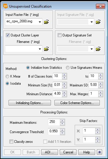Figure 1 This is the unsupervised classification tool window where the classification parameters are set.

Figure 2 The image on the left is the original 2009 image and the image on the right is the newly classified image.

Section 2: Recoding of unsupervised clusters into meaningful land use/land cover classes

Once we have the new unsupervised classification image the next step is to recode the clusters created into meaningful LULC classes. This is a pretty simple process however the more time spent can increase or decrease the classification accuracy. To recode we open the image attributes with the newly classified image open in ERDAS 2015. We go through each cluster and change the color to yellow one at a time so they stand out in the image. We then since the image to Google Earth so that we can see the actually features and surface in the cluster areas we have highlighted. Based on what we see in Google Earth for each cluster we label and change the color scheme. The labels that were  assigned to the clusters were Water which is changed to Blue, Forest is Dark Green, Agriculture is Pink, Urban/Buildup is Red and Bare Soil is Sienna. Figure 3 is the recoded unsupervised classification image with the new color assignments to each class.

Figure 3 This is the reclass image making use of only 10 classes. The class labels and associated colors can be seen in the table.

Part 2: Improving the accuracy of unsupervised classification 

Section 1: Setting up and running an unsupervised classification algorithm 

The second portion of the lab was very similar to the first. Again we are going to bring in the original aerial imagery from 2009. This time however in the classification window we are going to set the classes 20 to 20. This will increase the number of classes the algorithum splits the brightness values into, increasing accuracy. One other slight change is reducing the coverage threshold from .95 to .92. Once we have this new classified image with 20 classes instead of 10 we use the same procedure as in part 1 section 2 to assign the correct labels to each class as well as change the colors. Figure 4 is the newly reclassed image with the attributes showing the labels and colors.

Figure 4 This is the newly reclassed image using 20 classes to increase the accuracy. 

Section 2: Recoding LULC classes to enhance map generation 

The final piece to the lab is to combine the classes so that the LULC classes are easier to understand and displayed more effectively when creating a map. This was done only on the image with 20 classes from part 2. The 20 classes are recoded or combined by kind so there are only 5. In order to this the recode tool under the thematic tab is used. The class numbers were 1. Water  2. Forest 3. Agriculture 4. Urban/Builtup 5. Bare Soil. Figure 5 shows the 20 classes combined into 5 using the recode tool.  These values can then be used to create a LULC map in ArcGIS or another GIS software.

Figure 5 These are the 5 classes created using the recode tool. Each of these is multiple classes combined by type to go from 20 to 5 classes.

Results

There is a noticeable difference between the 10 class and 20 class unsupervised classification images (Figure 6). The most noticeable difference is between the forest and agricultural areas. Many of these areas were overlapping in the 10 class image so it was difficult to separate these areas into the correct class. The majority rules when choosing the classes to if there are more trees in the clustered area then it would be forest and the same is true for all the classes. It is much more generalized than the 20 class image where the clusters have a clear majority and it isn't as hard to separate them into the correct classes. One of the biggest factors in the accuracy is how much time the user spends comparing the clusters to Google Earth or other high res imagery to accurately separate the classes. If this is done quickly the classification most likely will not be accurate. Figure 7 is the final map created in ArcGIS using the recoded 5 class image.

Figure 6 These are the two reclassed images for comparison. The image on the left is the image split into 10 classes and the image on the right has 20 classes.

Figure 7 This is the final map created in ArcGIS.

Sources

The Landsat satellite imagery is from Earth Resources Observation and Science Center, United States Geological Survey.