Advanced Remote Sensing Lab 10 : Advanced Classifiers 3

Goals and Background

The main goal of this lab is to learn how to use two advanced classification algorithms. These advanced classifiers are very robust and can greatly increase the accuracy of the LULC classification. The main objectives for the lab are as follows:
1)  Show us how to perform an expert system/decision tree classification with the use of ancillary data
2) Demonstrate how to develop an artificial neural network to perform complex image classification

Methods

Part 1: Expert system classification 

 Section 1: Development of a knowledge base to improve an existing classified image

The first part of the lab is working with a method called expert system classification. This is a very robust classification method that uses not only the remotely sensed imagery but also ancillary data to get a more accurate final classification.

To begin we were given a classified image of the Chippewa Valley (Figure 1). We examined the image and found that there were a number of errors in the LULC classifications. These included urban areas that were labeled as residential when they were clearly industry and many agricultural areas were labeled as green vegetation and vise versa. These errors would be corrected by running this imagery again in the expert system classification to improve the accuracy and get a more realistic classification of the area.

Figure 1 This is a classified image of the Chippewa Valley with errors in the LULC classification.

The first step to running the expert system classification is to create hypothesis and rules for each of the classes we are interested in. To do so we open the knowledge engineer window. Figure 2 is what this window looks like. This was repeated for each of the six classes which are water, residential, forest, green vegetation, agriculture, and other urban.

Figure 2 This is the window to set up the rules for each of the hypothesis or classes in the knowledge file.

Section 2: The use of ancillary data in developing a knowledge base 

Once those 6 hypothesis or classes are entered the next step is to write an argument that will make sure that the other urban class does not get classified as residential urban. There are two arguments that are written one from the residential hypothesis saying that residential will not be classified as other urban and one by the other urban hypothesis saying that other urban will not be classified as residential. These arguments help the classifier better distinguish between the two classes. The same procedure was followed for green vegetation and agriculture. A argument was added to the agriculture saying that agriculture can not be classified as green vegetation and also the opposite is true that green vegetation can not be agriculture again to help the classifier separate those classes more accurately and correct the errors seen in the original classified image we examined. Figure 3 is the final process tree for the expert system classifier. This knowledge file saved for use in the next step of the lab.

Figure 3 This is the final process tree or knowledge file for the expert system classification.

Section 3: Performing expert system classification 

To run the expert the knowledge classifier window is opened once again and the knowledge file or Figure 3 is brought in. This is where you can select which hypothesis or classes you want to include in the classification. In this case we included all of them Figure 4. After the classes to include are selected click OK and the next window is opened (Figure 5). Here we set the cell size to 30 by 30 and select the location and name of the final output classified image. Hit OK and the classifier runs. Figure 11 is the final classified map.

Figure 4 We include all of the classes for this analysis. 

Figure 5 This is the dialogue box to pick the output location of the classified image as well as set some other parameters.

Part 2: Neural network classification 

Section 1: Performing neural network classification with a predefined training sample 

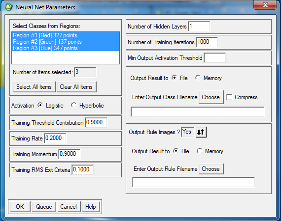
The other method of classification we explored in this lab is called Neural Network classification. This portion of the lab was run in ENVI 4.6.1 another remote sensing software. The first step was to open an image file provided by Dr. Cyril Wilson. Once the image was open the next step was to import an ROI file. These ROIs are training samples that Dr.Wilson collected in this imagery (Figure 6). Once the ROIs are open neural network classification is chosen from the supervised drop down in ENVI. Figure 7 is the parameter window for the classification where the number of iterations, training rate, and output location for the classified image are input. Once the parameters are entered the classification is run and Figure 8 is the result.

Figure 6 This is the image give to us by Dr. Wilson you can see that I have also brought in the ROIs on top of the image.

Figure 7 This is neural network dialogue box where the majority of the parameters are input.

Figure 8 The original false infrared image is on the left and the classified image is on the right.

Section 2: Creating training samples and performing NN classification (Optional challenge section) 

Additional practice and experimentation with the parameters for the neural network classification was done using an image of Northern Iowas campus (Figure 9). I opened the image and instead of having ROIs provided I created them myself. I made three classes which were grass, roofing, and concrete/asphalt. The same procedure for running the classification was followed as above. Figure 10 is the resulting classified image based on the 3 ROIs or classes I created.

Figure 9 This is the original false infrared image of the Northern Iowa campus.

Figure 10 This is the original image on the left and the classified image on the right based on the ROIs I collected.

Results

Figure 11 This is the final LULC map using the expert system classification method.

Sources

The Landsat satellite images are from Earth Resources Observation and Science Center, United States Geological Survey.
The Quickbird High resolution image of portion of University of Northern Iowa campus is from Department of Geography, University of Northern Iowa.