Advanced Remote Sensing: Lab 7 Digital change detection

Goals and Background

The main goal of this lab is to develop skills and get a better understanding of how to evaluate and measure changes that occur on land use and land cover over time. To do this digital change will be used which is an important tool for monitoring environmental and socioeconomic phenomena in remotely sensed images. There three objectives which fall under this digital change detection method. They are:

1)  how to perform quick qualitative change detection through visual means

2) quantify post-classification change detection

3) develop a model that will map detail from-to changes in land use/land cover over time

Methods

Part 1: Change detection using Write Function Memory Insertion 

The first portion of the lab makes use of Write Function Memory Insertion. This is a very simple yet effective method of visualizing changes in LULC over time. In order to do this the near-infrared bands from two images of the same area at different times are put into the red, green and blue color guns. When this is done the pixels that changed between those two time periods will be illuminated or be a bright color compared to the rest of the image and areas that did not change. These areas of change are then easy to see and get a quick overview of the change that has occurred between the two study times. In Figure 1 below you can see the areas highlighted in red that stand out from the rest of the the image. These are areas of change between 1991 and 2011.

Figure 1 Write Function Memory Insertion change image of Eau Claire County for 1991 to 2011.

Part 2: Post-classification comparison change detection

Section 1: Calculating quantitative changes in multidate classified images 

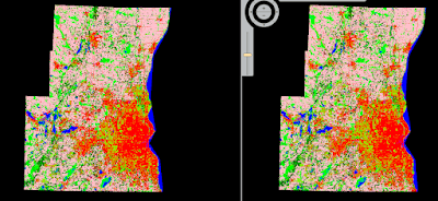
The next portion of the lab is about conducting change detection on two classified images of the Milwaukee Metropolitan Statistical Area (MSA). The two images being compared are from 2001 and 2011. The images were already classified and provided be Dr. Cyril Wilson. Figure 2 is the two MSA images side by side in ERDAS Imagine. 

Figure 2 These are the MSA classified images for 2001 right and 2011 on the left.

Once the two images were brought so we could visually compare the two the next step was to quantify the change between the two time periods. This was done by obtaining the the histogram values from the raster attribute table and then input those values into an excel spread sheet by class. These values are then converted to square meters and then from square meters to hectares. Once the we had the hectare values for each of the classes for 2001 and 2011 the percent change was calculated. This is done by taking the 2011 values and subtracting them from the 2001 and then multiplying that by 100. Figure 3 is the resulting table with the percent change values.

Figure 3 This table is showing the percent change for each LULC class from 2001 to 2011.

Section 2: Developing a From-to change map of multidate images 

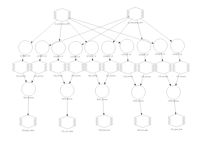
The final portion of this lab was to create a from-to-change map from the two MSA images. A model was created which detects the change between the two images. We made use of the Wilson-Lula algorithm. Figure 4 is the model that was created. In this model I focused on changes between 5 pairs of classes. Those 5 pairs are as follows: 1. Agriculture to urban 2. Wetlands to urban 3. Forest to urban 4. Wetlands to agriculture 5. Agriculture to bare soil. The first part of the model takes the two MSA images and separates them into the individual classes through an either or statement. Each class from the two years is then paired up based on the 5 pairs above. Once paired up the Bitwise function is used on each pair to show the areas that have changed from one LULC class to another over the time period. These 5 output rastersare then used to create a map of the changes that took place. Figure 5 is the final resulting from-to change map.

Figure 4 This is the from-to-change model making use of the Wilson-Lula algorithm to calculate LULC change from one class to another. 

Results

Figure 5 This is the final from-to-change map. Each are that is colored is showing a change in LULC class in the 5 pairings created earlier in the lab for use in the model in Figure 4.

Sources

The Landsat satellite image is from Earth Resources Observation and Science Center, United States Geological Survey. 

Homer, C., Dewitz, J., Fry, J., Coan, M., Hossain, N., Larson, C., Herold, N., McKerrow, A., VanDriel, J.N., and Wickham, J. 2007. Completion of the 2001 National Land Cover Database for the Conterminous United States. Photogrammetric Engineering and Remote Sensing, Vol. 73, No. 4, pp 337-341.

Xian, G., Homer, C., Dewitz, J., Fry, J., Hossain, N., and Wickham, J., 2011. The change of impervious surface area between 2001 and 2006 in the conterminous United States. Photogrammetric Engineering and Remote Sensing, Vol. 77(8): 758-762.

The Milwaukee shapefile is from ESRI U.S geodatabase.